 |
Prime I.T. | |
|
Help Prime I.T. : |
 Version Française
|
 Bitcoin adress
  Litecoin adress
  Dodgecoin adress
 The Euclidean division
The principle
This article discusses the Euclidean division, fundamental subject, representing
the starting point for all issues related to prime numbers and factorization of integers.
Euclidean division is with addition, subtraction and multiplication one of the four basic
operations on integers. Its purpose is to try to leave fairly a given group of elements
relative to a constraint characterized by a number.
For example a bag containing 12 balls to distribute over 3 people or the cake of grandma
cut into 8 portions while we are 6 around the table.
We consider in this article we work on positive integers (set N natural numbers), thus this
equitable distribution is sometimes impossible without the appearance of "halves", "quarters",
"third party" or other... For example 3 balls to be distributed over 2 people give each 1 ball
and we not try to cut the last... This residue undistributed is set aside, it is the rest.
Note that on rational numbers (set Q) and so on real numbers (very coarsely floating numbers)
the distribution is possible but can give something with difficulty representable in real life,
for example 10 / 3 = 3.3333... this means 3 up to infinity, difficult to cut a cake in these
conditions...
From a mathematical point of view, the definition of the Euclidean division for natural numbers
is as follows :
Let a and b be integers and b different from 0, there exists a unique pair (q, r) of integers
such as:
- a = bq + r
- r < b
Note 1 : We refind this notion of equitable distribution with the term "bq" and the
residue with the term "r".
Note 2 : For integers (set Z of integers positive and negative) we have almost the
same definition. Only the second condition changes and becomes |r| < |b|.
About name on the terms of the Euclidean division "a = bq + r", we have:
- a is the dividend
- b is the divisor
- q is the quotient
- r is the remainder
Implementation of tests
Throughout this article we will present some known implementations of Euclidean division and compare them to see which are the most effective and faster. But to assess the time and confront results, we should have a small test program that will measure the time of the different implementations of the division and also check the three criteria following to avoid bias in testing :
- The test sets must be consistent : one division being order of the millisecond, if we test just one division we can not extract relevant information because the time is too short. We will therefore do runs of 20 million divisions.
- The test sets must be identical for each implementation : to compare two implementations of the Euclidean division, it will be sure to use the same set of test because divide with different methods on different numbers has no interest.
- Make several test sets with different properties : the idea is to test implementations of the division on sets having different properties in order to push the strengths and weaknesses of the implementation.
The java class EuclideTestCaseGenerator is responsible for the generation of test sets. This
will create sets according to 3 methods : One named "random" will take randomly numbers a (the
dividend) and b (the divisor) between 1 et 1000 billion, another named "A > B" idem to
"random" except that a is necessarily greater than b and one last named "custom" same as random
with a > 4*b.
Finally, the java class EuclideBench is the orchestrator to launch implementations of the
Euclidean division. Implementations must implement (as java) interface IEuclide.
source
First implementation
The easiest way to calculate the Euclidean division is relying on its definition : "how many times can i put b in a ?". This results in an algorithm easy to do and relatively short consisting subtract many times as it can be b (the divisor) of a (the dividend), until obtain a remainder less than b.
long r = a;
long q = 0;
while (r >= b) {
r = r - b;
q = q + 1;
}
long[] euclide = { q, r };
return euclide;
}
For the moment we do not have any elements of comparison with other implementations but
believe me the method is naive :).
All that we can see on this algorithm is the risk of not result when a is too big relative to b
because the variable r in the instruction "r = r - b" not decreasing fast enough. The complexity
of the algorithm is O(a).
source
Second implementation
To improve the first implementation, it might be interesting to code decimal division that we
learn in school. And for those who do not remember how it works, we following a simple schema
that is much better that a long speech to remember the method... take care the schema shows
how learn young French. According to the corner of the world where you have studied the position
numbers and visual changes but overall principles remain the same :
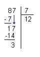 ie 87 = 7 * 12 + 3
At the implementation level, the method consists in multiplying b (the divisor) by 10 several
times as it is less than a (the dividend) then do the division identical to the first
implementation and finally, again with as dividend the remainder of the division of the
previous step.
long r = a;
long q = 0;
long n = 1;
long aux = 0;
while (r >= b) {
while (b * n <= a) {
n *= 10;
}
n /= 10;
aux = b * n;
while (r >= aux) {
r = r - aux;
q = q + n;
}
a = r;
n = 1;
}
long[] euclide = { q, r };
return euclide;
}
Throughout this article we will give results in the form of three tables representing a run
on each of the three test sets (Random, A > B et A > 4 * B). It is important to see that
the reading direction is from top to the bottom and the algorithms must be compared only in the
context of a run. Here we have taken randomly 40 million numbers (2 times 20 million) and
calculated the time taken by the naive and decimal algorithm to do 20 million Euclidean
divisions (This is the run 1). Then we took other numbers such as A > B and redo the 20
million divisions (run 2) then the same for A > 4 * B (run 3).
All that to say that there is few interest to compare 2 separate run because the data sets are
different while it is true that we see the time increases between the 3 runs, this growth is
difficult to quantify.
Let's see what happens.
| Random | A > B | A > 4 * B | |||||||
|---|---|---|---|---|---|---|---|---|---|
| Run / Check | n°1 / 150660990 | n°2 / 294686702 | n°3 / 1221575580 | ||||||
| Naive | 1.437 | 2.281 | 5.375 | ||||||
| Decimal | 2.0 | +0.563 | 2.984 | +0.703 | 4.032 | -1.343 | |||
This second implementation shows that the naive method is faster when we take random values
or when a (the dividend) is greater than b (the divisor) because the algorithm is very simple
and go fast. By cons when b is 4 times smaller than a, performance are reversed and the decimal
method becomes much faster.
On the test case A > B we may wonder why there is no gain, simply because the test set is
inadequate ! The problem comes from the distribution of numbers upon random shooting. For
example, if we choose a number between 0 and 1000 we have 89.99% chance of hitting a 4-digit
number (results can be extrapolated to n digits), on the 4-digit numbers we have ratios a / b
very low and so the result A > B is inconclusive. By adding the condition A > 4 * B we
increase artificially the ratio and we see clearly a gain.
The second algorithm is less dependent on the ratio a / b because we start by multiplying by
10 b as many times as necessary to be closer to a.
source
Third implementation
To optimize the computing time of the Euclidean division, we will change strategy by
implementing an algorithm based on the dichotomy. This method allows a very fast search of a
value using the good old adage "divide and conquer".
Here the dichotomic search will focus on the value of q (the quotient). The approach consist
first step to limit q, then repeatedly cutting into two equal parts this interval and selecting
the interval contains q.
It should be noted that these operations boundary and cutting will be done with powers of 2
or in other words, we use binary operations making it easier for a computer.
To find the first limit of q, we first find an n such that b * 2^n-1 <= a < b * 2^n,
that we can translate 2^n-1<= q <2^n.
Then we run the binary search before setting alpha = 2^n-1 et beta = 2^n
The dichotomy criteria are the following :
- If b * ((alpha + beta) / 2) <= a then alpha = (alpha + beta) / 2
- If b * ((alpha + beta) / 2) > a then beta = (alpha + beta) / 2
And it works ! Step by step we are getting closer (and finding) the quotient q. For more
details, including mathematical demonstration of the method, refer to the Wikipedia french
article on the Euclidean
division (binary method section). Unfortunately not found in English.
long n = 0;
long aux = b;
if (a < b) {
long[] euclide = { 0, a };
return euclide;
}
while (aux <= a) {
aux = (aux << 1);
n++;
}
long alpha = (1 << (n - 1));
long beta = (1 << n);
while (n-- > 0) {
aux = (alpha + beta) >> 1;
if ((aux * b) <= a) {
alpha = aux;
} else {
beta = aux;
}
}
long[] euclide = { alpha, a - (b * alpha) };
return euclide;
}
And we improve the performance...
With an approach of dichotomy we feel a "gap" has been crossed. As the decimal method allows
a large gain under the condition that a (the dividend) is very large compared to b
(the divisor), here we have the impression of a generalized gain on all test sets. And this is
normal because we passed log2(a).
source
| Random | A > B | A > 4 * B | |||||||
|---|---|---|---|---|---|---|---|---|---|
| Run / Check | n°4 / 198332981 | n°5 / 394652967 | n°6 / 1390554002 | ||||||
| Naive | 1.578 | 2.75 | 5.921 | ||||||
| Decimal | 2.0 | +0.422 | 3.0 | +0.25 | 4.032 | -1.889 | |||
| Binary dichotomy | 1.375 | -0.625 | 2.015 | -0.985 | 3.297 | -0.735 | |||
Fourth implementation
Always looking for performance, we make a great leap backward in the history of civilization
as we are going to inspire from the technical division in ancient Egypt to implement the fourth
of the Euclidean division algorithm.
Question : Were Egyptians at the time of the pharaohs all potential computer scientist ?
Nobody knows but their techniques of multiplication
and division
relied mainly on the decomposition numbers in powers of 2 in order to make these 2 operations.
Basically they reasoned in binary to able to multiply and divide.
- About multiplication, the goal was to transform in binary the first operator (see
Wikipedia for this transformation) and then build the table of powers of 2 multiplied by the
second operator (easy, simply multiply by 2 the 2nd operator as many times as you wish), and
finally summing the values in the table as "where there is a bit setted".
Example with 18 * 9 = ? 18 (binary) 9 * 2 (n times) 0 9 1 18 there is 1, we pick 0 36 0 72 1 144 there is 1, we pick So 18 + 144 = 162 = 18 * 9.
- About division, Egyptians used the same principle but in reverse.
They began by building the table of powers of 2 multiplied by the divisor (always with a multiplication by 2)until arriving at a number greater than a (the dividend). Then they rebuilding "the result in binary" by selecting the numbers such as their additions do not exceed a. This selection starting from the largest number (the highest bit).
Example 218 / 6 = ? n 6 * 2 (n times) Addition 5 192 192 we pick because 192 < 218 4 96 X we don't pick because 192 + 96 = 288 et 288 > 218 3 48 X we don't pick because 192 + 48 > 218 2 24 216 we pick because 192 + 24 = 216 et 216 < 218 1 12 X we don't pick because 216 + 12 > 218 0 6 X we don't pick because 216 + 6 > 218 So 192 + 24 = 216, ie 6 * (2 ^ 5) + 6 * (2 ^ 2) = 216.
The quotient q is 2 ^ 5 + 2 ^ 2 = 36, the remainder r is 2 (218 - 116).
The majority of sites on the web speak of the Egyptian division as an historical approach and not as computer science. Thus we find the operating principle and a lot of informations describing the subject in textual form. By cons we have not seen an example of implementation of the algorithm, but that does not matter, just do it !
long n = 0;
long p = b;
if (a < b) {
long[] euclide = { 0, a };
return euclide;
}
while (p <= a) {
p = (p << 1);
n++;
}
p = (p >> 1);
n--;
long q = (1 << n);
long aux = p;
while (n > 0) {
p = (p >> 1);
n--;
if ((aux + p) <= a) {
q += (1 << n);
aux += p;
}
}
long[] euclide = { q, a - aux };
return euclide;
}
About variable, we have :
- p : representative of the calculations on b * 2 ^ n (the second column in example) on which we do our multiplication and division by 2 via a "shift".
- aux : representing the sum that should not exceed the dividend (third column in the example).
We note that the algorithm is very similar to the binary division by dichotomy, especially the first part
where we need to look for n in order to limit a (the dividend) such as
b * 2^n-1 <= a < b * 2^n but also the loop "while (n > 0)" in center of the program.
In fact, these two algorithms are equivalent, one that can be written in another.
source
In terms of performance, we gain again more speed. Certainly not as much as the change from
decimal to dichotomous but gain of 0.2s (except random) on average is honorable.
| Random | A > B | A > 4 * B | |||||||
|---|---|---|---|---|---|---|---|---|---|
| Run / Check | n°7 / 162438146 | n°8 / 313167294 | n°9 / 1211389641 | ||||||
| Naive | 1.406 | 2.781 | 5.5 | ||||||
| Decimal | 2.016 | +0.61 | 3.0 | +0.219 | 3.828 | -1.672 | |||
| Binary dichotomy | 1.39 | -0.626 | 2.0 | -1.0 | 3.015 | -0.813 | |||
| Binary egyptian | 1.36 | -0.03 | 1.781 | -0.219 | 2.719 | -0.296 | |||
Fifth implementation
And here is the latest implementation of the Euclidean division, it is the method
of binary dichotomy supplemented with Horner method.
In fact, it is simply a more elegant rewriting of the Egyptian division (fourth
implementation) which itself is equivalent to the third (if you follow...).
long r = a;
long q = 0;
long n = 0;
long aux = b;
while (aux <= a) {
aux = (aux << 1);
n++;
}
while (n > 0) {
aux = (aux >> 1);
n--;
q = (q << 1);
if (r >= aux) {
r = r - aux;
q++;
}
}
long[] euclide = { q, r };
return euclide;
}
In performance is less good on our old test computer AMD 3200 2 Ghz than
the implementation of the Egyptian division, to see if on other machines (or other
languages) we have also this difference.
source
| Random | A > B | A > 4 * B | |||||||
|---|---|---|---|---|---|---|---|---|---|
| Run / Check | n°10 / 394782450 | n°11 / 411583635 | n°12 / 1593795009 | ||||||
| Naive | 2.828 | 2.859 | 6.562 | ||||||
| Decimal | 3.031 | +0.203 | 3.078 | +0.219 | 4.031 | -2.531 | |||
| Binary dichotomy | 2.125 | -0.906 | 2.078 | -1.0 | 3.313 | -0.718 | |||
| Binary egyptian | 1.829 | -0.296 | 1.844 | -0.234 | 3.015 | -0.298 | |||
| Binary | 2.046 | +0.217 | 2.031 | +0.187 | 3.172 | +0.157 | |||
In conclusion
So, this concludes the presentation of some algorithms Division Euclidean.
We note that we saw 5 implementations, which is a high number, but it is
likely that there are more other non-commented and/or not visible.
